Vision Transformers are Overrated
Vision transformers (ViTs) have seen an incredible rise in the past four years. They have an obvious upside: in a visual recognition setting, the receptive field of a pure ViT is effectively the entire image 1. In particular, vanilla ViTs maintain the quadratic time complexity (w.r.t. number of input patches) of language models with dense attention.
Kernels in convolutional networks, on the other hand, have the property of being invariant to the input pixel/voxel that it is applied to, a feature that is typically referred to as translation equivariance. This is desirable because it allows the model to effectively recognize patterns and objects regardless of where they are located spatially. The weight sharing present in convolutional layers also makes convnets highly parameter-efficient and less prone to overfitting - a property ViTs do not have.
As such, you might expect that ViTs and convnets are used equally in production environments that leverage visual models - ViTs for “global” tasks such as scene recognition and convnets for more “local” tasks such as object recognition. Even so, we’ve been inundated with work that utilizes ViTs, with bold high-level claims (mostly by media outlets) that convnets are a thing of the past.
Curious to see if I could lend a hand in helping debunk this claim, I set out to figure whether or not a mostly vanilla ResNet could match or even exceed the performance of both ViT and ConvNeXt. The comparison to ConvNeXt is of particular interest, since it is a fully convolutional network that attempts to bridge the gap between transformers and convnets.
With a bit of experimentation on Imagenet-1k, we can reach 82.0% accuracy with a 176x176 training image size with no extra data, matching ConvNeXt-T (v1, without pre-training a-la MAE) and surpassing ViT-S (specifically, the ViT flavor from DeiT-III).
Training methodology
We start by adopting the training methodology set in Pytorch’s late 2021 blog, where they achieved an impressive 80.8% accuracy on Imagenet-1k with a stock ResNet50 model. Here’s a couple of key points to note:
- We stick with SGD as the optimizer, rather than going for RMSProp or Adam (or any of their variants).
- The scheduler uses cosine decay with five warmup epochs and 600 total epochs. This may seem like an unnecessarily large number of epochs, but we’ll get around to reducing this later.
- We utilize a whole slew of augmentations found in modern literature, including, but not limited to: label smoothing, mixup, cutmix, and model EMA.
- To prevent overfitting on the validation dataset, we’ll skip hyperparameter tuning and grid search and stick with the stock training methodology listed out in the blog post.
Nearly all of these training optimizations have already been used to boost the performance of modern visual recognition models, but adopting these changes don’t quite get us to the magical 82% accuracy we’re looking for.
Architectural modifications
The baseline ResNet architecture is strong but not optimal, so we adopt a few architectural modifications to enable better performance:
ResNet-d
First order of business is the embrace some “modernizations” to ResNet. For completeness, here are the changes listed out:
- The initial 7x7 convolution is changed to a sequence of three 3x3 convolutions with 32, 64, and 128 output channels, respectively. The stride remains on the first convolutional layer. With this change, we now use exclusively 3x3 and 1x1 convolutions across the entire network all while retaining the original size of the receptive field for the network head.
- Strides in downsampling residual blocks are moved from the first 1x1 convolutional layer to the subsequent 3x3 convolutional layer. This has the effect of capturing all input pixels in a downsampling block, since a strided 1x1 convolution effectively skips every other pixel.
- The max pooling in the stem is removed. The first 3x3 convolution of the first residual block now has a stride of two, matching the remaining residual blocks. While max pooling is theoretically useful for retaining edges, corners, and other low-level features, I haven’t found it to be particularly useful in practice.
- The strided 1x1 convolution in the shortcut connections of downsampling blocks is replaced with 2x2 average pooling followed by a standard 1x1 convolutional layer. Again, this has the effect of capturing all input activations rather than just one out of every four input channels.
The resulting micro-optimizations result in an architecture that is extremely close to ResNet-d, with some very minor differences.
ReLU -> SiLU
ReLU has two weaknesses compared to other activation functions: 1) it is not smooth (ReLU is, strictly speaking, non-differentiable at 0), and 2) the “dying ReLU” problem, where pre-activation values are near-universally negative during a forward pass, causing gradients to always be zero and the neuron to carry no information. As a direct result, a number of novel activations have been proposed throughout the years - Leaky ReLU, Parametric ReLU, ELU, and Softplus are three well-known albeit older examples. The idea behind all of these is to fix one or both of the above problems; Parametric ReLU, for example, attempts to fix the dying ReLU problem by introducing a learnable parameter $\alpha$ that defines the slope the function for negative pre-activation values. For this model, I went with the SiLU, (also commonly known as Swish), defined by $SiLU(x) = \frac{x}{1+e^{-x}}$, which has already seen success with a number of visual recognition models. Since this switch enabled faster training, I reduced the number of epochs from 600 to 450.
Although I could’ve used GELU, I decided to use SiLU because it has an inplace parameter and could serve as a drop-in replacement for ReLU in the original reference implementation. GELU or GLU variants (SwiGLU, GeGLU) might have performed slightly better as they are widely used in language models. Although GELU and SiLU are highly correlated 2, networks trained with GELU are not equivalent to networks trained with SiLU in terms of representational capacity due to differences in weight decay and initialization.
Lastly, I hypothesize that a SiLU network would likely perform better with stochastic depth since ReLU may act like a weak implicit regularizer by adding sparsity to the network activations. This can be great for overparameterized models, but not for parameter-efficient models. SiLU, on the other hand, has nonzero gradients for all values $x$ except for $x \approx -1.278$. As such, with the switch from ReLU to SiLU, adding a bit of regularization might be warranted. I’ll have to experiment more with this in the upcoming weeks.
Update (03/23/2024): After some experimentation, I found that stochastic depth with a drop probability of 0.1 negatively impacts the performance of the network (by about 0.2% or so), but reducing it to 0.05 results in what is effectively the same accuracy. I’ll need to play around with it a bit more.
Split normalization
Vanilla ResNet uses a generous amount of batch normalization (BN); one BN layer per convolutional layer to be exact. The original BN paper argues that BN improves internal covariate shift (ICS) - defined by the authors as the change any intermediate layer sees as upstream network weights shift - but this has since proven to be untrue (I’ll elaborate on this in a bit). I wanted to go back to the original ICS thesis, i.e. normalization in BN was meant to re-center the activations, while the learnable affine transformation immediately following normalization was meant to preserve each layer’s representational capacity. It simply made no sense to me that these two must be applied back-to-back. Furthermore, since backpropogation effectively treats each individual layer of neurons as an independent learner, the most sensible thing to do is to normalize layer inputs rather than outputs.
Long story short, I found that splitting BN into two separate layers - pre-convolution normalization and post-convolution affine transformation - improves the network’s performance by over 0.4%. While this does negatively affect speed and memory consumption during training, it has zero impact on inference performance since the normalization and affine transformations can be represented as diagonal matrices and fused with the weights of the convolutional layer once the network is fully trained.

Split normalization, visualized.
I wanted to better understand the theory behind “split” normalization but couldn’t find it anywhere in ML literature3. As a result, I looked towards BN theory first; the most compelling research in my eyes comes from Santurkar et al.’s 2018 paper. In it, they show that BN often increases ICS. Instead, they argue that batch normalization works well because improves the first- and second-order properties of the loss landscape.
Through a quick exercise, we can show that split normalization (SN) has the same effect. Let’s consider two networks - one without SN defined by loss function $L$ and one with SN defined by loss function $\hat{L}$. For the network with SN, the gradients through each of these layers is as follows:
\[\begin{aligned} \frac{\partial\hat{L}}{\partial y_i} &= \frac{\partial\hat{L}}{\partial \hat{y}_i}\gamma \\ \frac{\partial\hat{L}}{\partial\hat{x}_i} &= \mathbf{W}^T\frac{\partial\hat{L}}{\partial\hat{y}_i} \\ \frac{\partial\hat{L}}{\partial x_i} &= \frac{1}{\sigma}\frac{\partial\hat{L}}{\partial\hat{x}_i} - \frac{1}{m\sigma}\sum_{k=1}^{m}\frac{\partial\hat{L}}{\partial\hat{x}_k} - \frac{1}{m\sigma}\hat{x}_i\sum_{k=1}^{m}\frac{\partial\hat{L}}{\partial\hat{x}_k}\hat{x}_k \end{aligned}\]Where $m$ is the size of each mini-batch and $y_i$, $\hat{y}_i$, $\hat{x}_i$, $x_i$ represent the activations for the $i$th sample in our batch. In practice, the dimensionality of the activation tensors can be arbitrarily large or small (e.g. 3d for most convnets). With this, we can represent the full loss gradient via dot products:
\[\begin{aligned} \frac{\partial\hat{L}}{\partial\mathbf{x}} &= \frac{\gamma}{m\sigma}\mathbf{W}^T\left(m\frac{\partial\hat{L}}{\partial\mathbf{y}} - \mathbf{1} \cdot \frac{\partial\hat{L}}{\partial\mathbf{y}} - \mathbf{x} \left(\frac{\partial\hat{L}}{\partial\mathbf{y}} \cdot \mathbf{x}\right)\right) \end{aligned}\]For a function $f(a)$, the L2 norm of its gradient $\left\Vert\frac{df}{da}\right\Vert$ is a good proxy for Lipschitzness. The same holds our loss function, i.e. we would like to show that $\left\Vert\frac{\partial\hat{L}}{\partial\mathbf{x}}\right\Vert \leq \left\Vert\frac{\partial L}{\partial\mathbf{x}}\right\Vert$. Given a matrix $\mathbf{A}$ and vector $\mathbf{b}$, the norm of the two multiplied together is bound above by the largest singular value of $\mathbf{A}$, i.e. $\Vert\mathbf{A}\cdot\mathbf{b}\Vert \leq s_{max}(\mathbf{A})\Vert\mathbf{b}\Vert = \sqrt{\lambda_{max}(\mathbf{W}^T\mathbf{W})}\Vert\mathbf{b}\Vert$. Given this, we have:
\[\begin{aligned} \left\Vert\frac{\partial\hat{L}}{\partial\mathbf{x}}\right\Vert^2 &\leq \left(\frac{\gamma}{m\sigma} \right)^2 s_{max}(\mathbf{W})^2\left\Vert m\frac{\partial\hat{L}}{\partial\mathbf{y}} - \mathbf{1} \cdot \frac{\partial\hat{L}}{\partial\mathbf{y}} - \mathbf{x} \left(\frac{\partial\hat{L}}{\partial\mathbf{y}} \cdot \mathbf{x}\right)\right\Vert^2 \end{aligned}\]Applying the reduction from C.2 in Santurkar et al., we get:
\[\begin{aligned} \left\Vert\frac{\partial\hat{L}}{\partial\mathbf{x}}\right\Vert^2 &\leq \frac{\gamma^2s_{max}^2}{\sigma^2} \left( \left\Vert \frac{\partial L}{\partial\mathbf{y}}\right\Vert^2 - \frac{1}{m}\left\Vert\mathbf{1} \cdot \frac{\partial L}{\partial\mathbf{y}}\right\Vert^2 - \frac{1}{m}\left\Vert\frac{\partial L}{\partial\mathbf{y}} \cdot \mathbf{x}\right\Vert^2 \right) \end{aligned}\]In my eyes, we should separate the multiplicative term (i.e. $\frac{\gamma^2s_{max}^2}{\sigma^2}$) from the additive term (i.e. $- \frac{1}{m}\left\Vert\mathbf{1} \cdot \frac{\partial L}{\partial\mathbf{y}}\right\Vert^2 - \frac{1}{m}\left\Vert\frac{\partial L}{\partial\mathbf{y}} \cdot \mathbf{x}\right\Vert^2$) since a) the multiplicative effects can be counteracted by increasing or decreasing the learning rate and b) $\mathbf{W}$ tends to change much slower than other terms in the equation. In particular, the additive term is strictly negative, which means that the overall loss landscape is smoother, while the potentially large multiplicative upper bound implies that SN may, in certain situations, be increasing the Lipschitz constant of the loss. At the same time, ICS at the inputs of each layer is strictly decreased, as the learnable affine transformation now comes after the weights rather than before.
The results
The final 26M parameter model successfully reaches 82.0% accuracy on Imagenet-1k without any external sources of data! In the spirit of modern machine learning research, let’s give this network a fancy name: GResNet (Good/Great/Gangster/Godlike ResNet).
| Model | Accuracy | Params | Throughput |
|---|---|---|---|
| GResNet | 82.0%* | 25.7M | 2057 im/s |
| ConvNeXt | 82.1% | 28.6M | 853 im/s |
| ViT (DeiT) | 81.4% | 22.0M | 1723 im/s |
Comparison of different models. Throughput calculated on a single Nvidia A100 with batch size 256 without network optimizations. *Accuracy improves to 82.2% and throughput drops to 1250 im/s when we use ConvNeXt's train image size of 224x224 instead of 176x176.
The GResNet model definition is available here, while weights are available here.
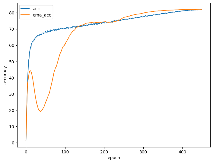
Accuracy curve during training.
Ending words
What exactly have we shown here? With some simple modifications to ResNet, we can attain excellent performance - on par or better than both ViT and a ViT-inspired convnet (ConvNeXt) on smallish datasets.
ConvNets never die, they just Transform
— Peyman Milanfar (@docmilanfar) October 27, 2023
ResNet strikes back... again?
You might be asking: why Imagenet-1k? Aren’t there a number of much larger labelled visual datasets i.e. YFCC, LAION, etc? Secondly, since modern LLMs are exclusively transformer-based, isn’t it beneficial to also use transformers for vision in order to take advantage of cross-attention or by linearly projecting patches into the decoder? The answer is yes: for large multimodal models bound by text, self-attention reigns supreme. But small models (e.g. most embedding models) are arguably more important because of their portability and adaptability, and these models benefit greatly from the exact type experiment of outlined in this post: strong augmentation with limited data trained across many epochs. This is exactly the type of data that Imagenet-1k represents.
And on the topic of ViTs being superior to convnets on large datasets: the 2023 paper titled Convnets match vision transformers at scale from folks at Google DeepMind is worth a read. The concluding section contains a stark result: “Although the success of ViTs in computer vision is extremely impressive, in our view there is no strong evidence to suggest that pre-trained ViTs outperform pre-trained ConvNets when evaluated fairly.” This simply reinforces a lesson that ought to be repeated: optimizations to model architecture should always come after 1) a large, high-quality dataset, 2) a solid, highly parallelizable training strategy, and 3) having lots of H100s. I’d argue that the bulk of transformers’ success has come from their ability to be efficiently and effectively scaled to hundreds of billions of parameters - scaling that could theoretically also be done with RNNs if research scientists had decades of time to train them (spoiler: they don’t).
Addendum - comparing embedding quality
I thought it might be interesting to compare embeddings from GResNet, ConvNeXt, and ViT by storing and indexing the embeddings from each model in Milvus:
>>> from milvus import default_server
>>> from pymilvus import MilvusClient
>>> default_server.start()
>>> client = MilvusClient(uri="http://127.0.0.1:19530")
>>> # initialize model, transform, and in1k val paths
...
>>> with torch.no_grad():
...     for n, path in enumerate(paths):
...         img = Image.open(path).convert("RGB")
...         feat = gresnet(transform(img).unsqueeze(0))
...         client.insert(collection_name="gresnet", data=[feat])
...
>>>
I removed the model initialization and data loading snippets for brevity and used Euclidean/L2 as the distance metric with no indexing (i.e. FLAT). With that step done, we can then query the collections to get results that look like this:
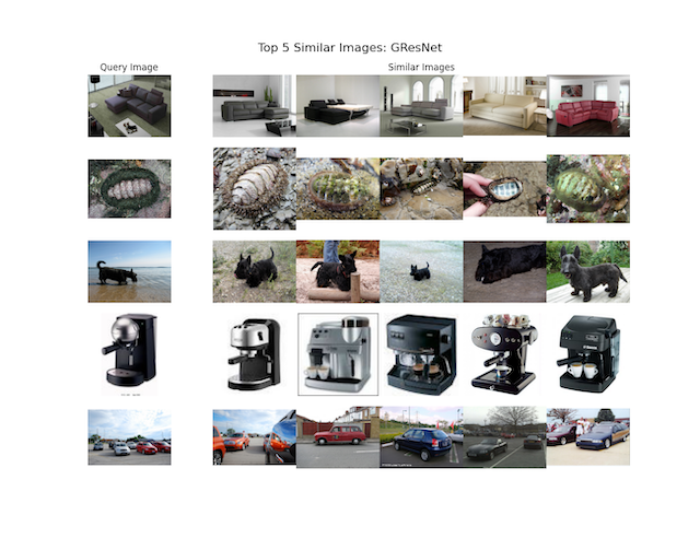
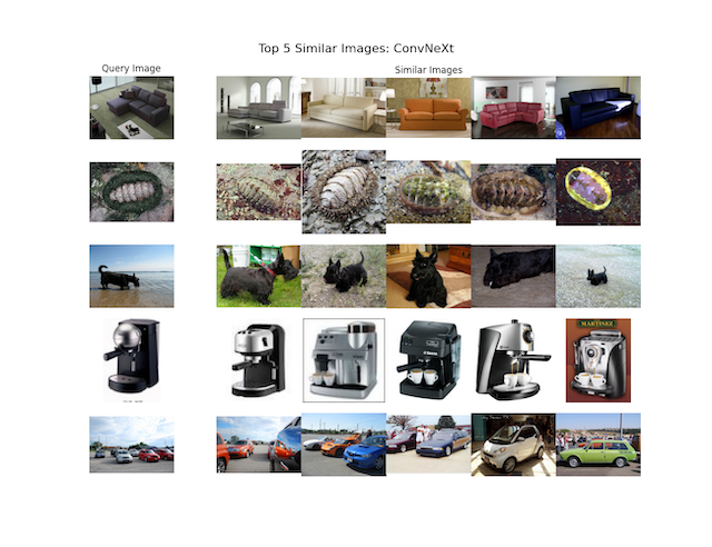
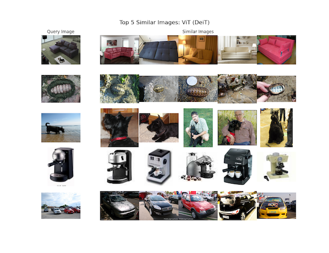
One could argue that GResNet tends to pick out images which are stylistically closer to the query image in addition to being the same class, but aside from that, the results between all three models are very comparable.
-
For a visual recognition model, the receptive field is the effective area of the input Nd-xels that a layer or neuron “sees” and can capture. Early layers in a pure convolutional model, for example, have a very small receptive field, while each layer in a vision transformer with dense attention sees the entire input image. ↩
-
There exists a fairly accurate approximation that relates GELU and SiLU: $GELU(x) = \frac{SiLU(1.702x)}{1.702}$. ↩
-
Please reach out to me if you know of prior work that implements this so I can give it a proper citation. ↩