Hierarchical Navigable Small Worlds (HNSW)
(Note: A version of this post has been cross-published to the Zilliz blog)
In a previous blog, we took a look at scalar quantization and product quantization - two indexing strategies which are used to reduce the overall size of the database without reducing the scope of a search. To better illustrate how scalar quantization and product quantization works, we also implemented our own versions in Python.
In this tutorial, we’ll build on top of that knowledge by looking at what is perhaps the most commonly used primary algorithm today: Hierarchical Navigable Small Worlds (HNSW). HNSW performs very well when it comes to both speed and accuracy, making it an incredibly robust vector search algorithm. Despite it being popular, understanding HNSW can be a bit tricky. In the next couple of sections, we’ll break down HNSW into its individual steps, developing our own simple implementation along the way.
HNSW basics
Recall from a previous post that there are four different types of vector search indexes: hash-based, tree-based, cluster-based, and graph-based. HNSW fits firmly into the lattermost, combining two core concepts together - the skip list and Navigable Small World (NSW). Let’s first dive into these two concepts individually before discussing HNSW.
Skip list overview
First up: skip lists. Recall the venerable linked list - a well-known data structure where each element in the list maintains a pointer the the next element. Although linked lists work great for implementing LIFO and FIFO data structures such as stacks and queues, a major downside is their time complexity when it comes to random access: O(n). Skip lists aim to solve this problem by introducing additional layers, allowing for O(log n) random access time complexity. By incurring extra memory (O(n log n) space complexity as opposed to O(n) for a normal linked list) and a bit of runtime overhead for inserts and deletes.
A skip list is essentially a multi-level linked list, where the upper levels maintain long connections. As we move down the layers, the connections become shorter and shorter, with the bottommost layer being the “original” linked list containing all of the elements. The image below illustrates this:
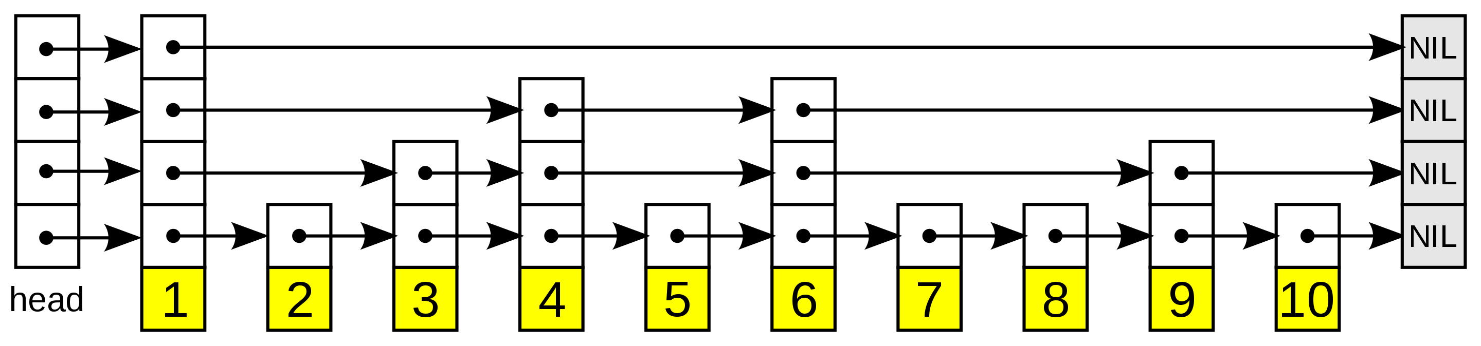
The skip list, illustrated. Higher layers have fewer elements.
To reach element i in a skip list, we first start at the highest layer. Once we find a node that corresponds to an element in the list that is greater than i, we then backtrack to the previous node and move to the layer below. This continues all the way until we’ve found the element we’re looking for. Note that skip lists only work for sorted lists, as we need a way to directly compare the magnitude of two objects.
Inserts work probabilistically. For any new element, we first need to figure out the layer with which the element appears first. The uppermost layer has the lowest probability, with increasing probability as we move down in layers. The general rule is that any element in a layer will appear in layer above it with some pre-defined probability p. Therefore, if an element first appears in some layer l, it will also get added to layers l-1, l-2, and so on.
Note that, while it is possible to have a terribly balanced skip list that performs no better than a standard linked list, the probability of this happening is incredibly low.
What the heck is a Navigable Small World?
Now that we’ve gotten skip lists out of the way, let’s take some time to talk about Navigable Small Worlds. The general idea here is to first imagine a large number of nodes in a network. Each node will will have short-, medium-, and long-range connections to other nodes. When performing a search, we’ll first begin at some pre-defined entry point. From there, we’ll evaluate connections to other nodes, and jump to the one closest to the one we hope to find. This process repeats until we’ve found our nearest neighbor.
This type of search is called greedy search. For small NSWs in the hundreds or thousands of nodes, this algorithm works, but it tends to break down for much larger NSWs. We can fix this by increasing the average number of short-, medium-, and long-range connections for each node, but this increases the overall complexity of the network and results in longer search times. In the absolute “worst” case, where each node is connected to every other node in our dataset, NSW is no better than naïve (linear) search.
NSWs are cool and all, but how does this relate to vector search? The idea here is to imagine all vectors in our dataset as points in an NSW, with long-range connections being defined by vectors which are dissimilar from one another and the opposite for short-range connections. Recall that vector similarity scores are measured with a similarity metric - typically L2 distance or inner product for floating point vectors and Jaccard or Hamming distance for binary vectors.
By constructing an NSW with dataset vectors as vertices, we can effectively perform nearest neighbor search by simply greedily traversing the NSW towards vertices closer and closer to our query vector.
HNSW, explained
When it comes to vector search, we often have dataset sizes in the hundreds of millions or even billions of vectors. Plain NSWs are less effective at this scale, so we’ll need a better graph.
HNSW extends NSW by borrowing from the concept of skip lists. Like the skip list, HNSW maintains multiple layers (hence the term Hierarchical Navigable Small World), only of NSWs instead of linked lists. The uppermost layer of an HNSW graph has few nodes and the longest links, while the bottommost layer has all nodes and the shortest links. During the search process, we enter a pre-defined point in the uppermost layer and greedily route ourselves towards the nearest neighbor to our query vector. Once we reach the nearest node, we then move to the second layer and repeat this process. This continues until we’ve reached our nearest neighbor.
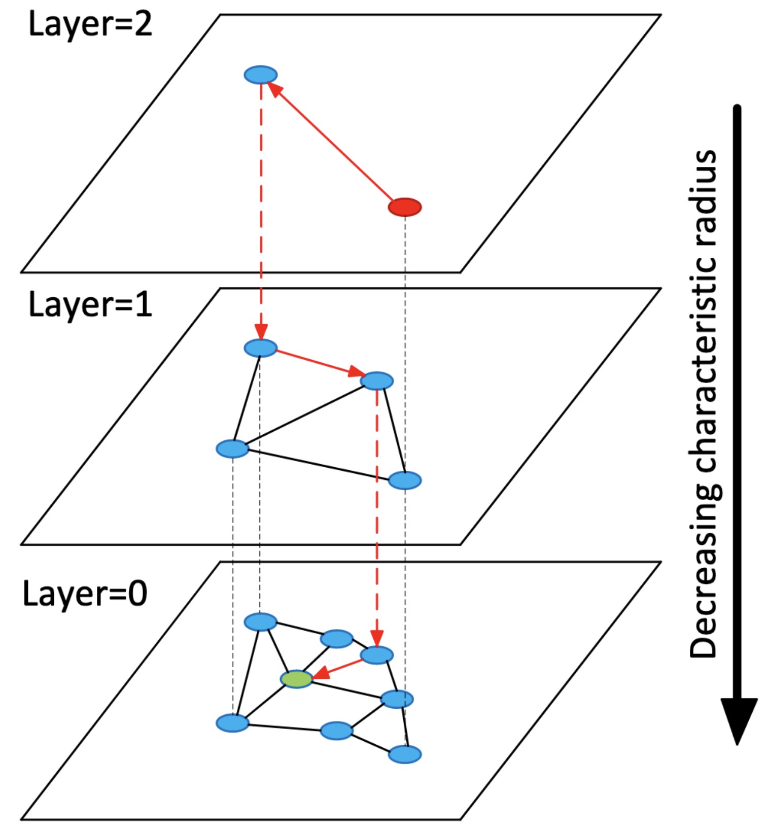
A diagram from the HNSW paper which visualizes the layered graph concept.
Inserts work similarly to the skip list. For some vector v, We first traverse the first layer of the graph, finding its nearest neighbor before moving to the layer below it. We then traverse the graph again to find its nearest neighbor in the second layer. This process until we’ve reached the nearest neighbor in the bottommost graph.
From here, we then need to determine which links (connections between vertices) to create. Again, we have a pre-defined parameter M which determines the maximum number of bidirectional links that we can add. These links are usually simply set as the nearest neighbors to v, but other heuristics can be used as well. The same process then repeats for the upper layers, assuming the vector appears there.
As with the skip list, the query vector will appear in upper layers with exponentially decreasing probability. Specifically, the HNSW paper uses the equation floor(-ln(rand(0, 1))), where rand(0, 1) is a random number sampled from a uniform distribution between (0, 1]. Note how this does not actually constrain the minimum distance between any two vertices/vectors in a particular layer - it’s entirely possible that we end up with a poorly constructed graph, but the probability that this happens is incredibly low, especially as we scale up the number of vectors in the HNSW index.
Implementing HNSW
HNSW is not trivial to implement, so we’ll implement only a very basic version here. As usual, let’s start with creating a dataset of (128 dimensional) vectors:
>>> import numpy as np
>>> dataset = np.random.normal(size=(1000, 128))
The first step is to build the HNSW index. To do so, we’ll need to add each vector in our dataset one-by-one. Let’s first create a data structure to hold our index. In this basic example, we’ll use a list of lists to represent the index, with the inner lists corresponding to each layer/graph:
>>> L = 5  # 5-layer HNSW
>>> index = [[] for _ in range(L)]
Every element in each graph is a 3-tuple containing the vector, a list of indexes that the vector links to within the graph, and the index for the corresponding node in the layer below it. For the bottommost layer, the third element of the 3-tuple will be set to None.
Since every insert first requires a search for the nearest neighbor in graph, let’s implement that first. We can traverse any of the subgraphs in the index as so:
def _search_layer(graph, entry, query, ef=1):

    best = (np.linalg.norm(graph[entry][0] - query), entry)

    nns = [best]
    visit = set(best)  # set of visited nodes
    candid = [best]  # candidate nodes to insert into nearest neighbors
    heapify(candid)

    # find top-k nearest neighbors
    while candid:
        cv = heappop(candid)

        if nns[-1][0] > cv[0]:
            break

        # loop through all nearest neighbors to the candidate vector
        for e in graph[cv[1]][1]:
            d = np.linalg.norm(graph[e][0] - query)
            if (d, e) not in visit:
                visit.add((d, e))

                # push only "better" vectors into candidate heap
                if d < nns[-1][0] or len(nns) < ef:
                    heappush(candid, (d, e))
                    insort(nns, (d, e))
                    if len(nns) > ef:
                        nns.pop()

    return nns
This code snippet is a bit more involved, but it’s much easier to understand with a bit of explanation. Here, we use a heap to implement a priority queue, which we use to order nearest neighbor vectors in the graph. Like all of the previous examples, I’m using L2 distance here, but this code can be extended to other distance metrics as well. We first populate the heap with the entry point.
Here, all we’re doing is implementing greedy search. At every iteration, our goal is to update two variables: nns, our output list of nearest neighbors, and candid, a heap of candidate points. We evaluate all nearest neighbors to the “best” vector in candid, adding better (better means closer to the query vector) vectors to the output list of nearest neighbors as well as to the heap of candidate points for evaluation on the next iteration. This repeats until one of two stopping conditions is reached: we either run out of candidate points to evaluate, or we’ve determined that we can no longer do any better than what we already have.
With top-k graph search out of the way, we can now now implement the top-level search function for searching the entire HNSW index:
def search(index, query, ef=1):

    # if the index is empty, return an empty list
    if not index[0]:
        return []

    best_v = 0  # set the initial best vertex to the entry point
    for graph in index:
        best_d, best_v = _search_layer(graph, best_v, query, ef=1)[0]
        if graph[best_v][2]:
            best_v = graph[best_v][2]
        else:
            return _search_layer(graph, best_v, query, ef=ef)
We first start at the entry point (zeroth element in the uppermost graph), and search for the nearest neighbor in each layer of the index until we reach the bottommost layer. Recall that the final element of the 3-tuple will resolve to None if we are at the bottommost layer - this is what the final if statement is for. Once we reach the bottommost layer, we search the graph using best_v as the entry point.
Let’s go back go the HNSW insert. We’ll first need to figure out which layer to insert our new vector into. This is fairly straightforward:
def _get_insert_layer(L, mL):
    # ml is a multiplicative factor used to normalized the distribution
    l = -int(np.log(np.random.random()) * mL)
    return min(l, L)
With everything in place, we can now implement the insertion function.
def insert(self, vec, efc=10):

    # if the index is empty, insert the vector into all layers and return
    if not index[0]:
        i = None
        for graph in index[::-1]:
            graph.append((vec, [], i))
            i = 0
        return

    l = _get_insert_layer(1/np.log(L))

    start_v = 0
    for n, graph in enumerate(index):

        # perform insertion for layers [l, L) only
        if n < l:
            _, start_v = _search_layer(graph, start_v, vec, ef=1)[0]
        else:
            node = (vec, [], len(_index[n+1]) if n < L-1 else None)
            nns = _search_layer(graph, start_v, vec, ef=efc)
            for nn in nns:
                node[1].append(nn[1])  # outbound connections to NNs
                graph[nn[1]][1].append(len(graph))  # inbound connections to node
            graph.append(node)

        # set the starting vertex to the nearest neighbor in the next layer
        start_v = graph[start_v][2]
If the index is empty, we’ll insert vec into all layers and return immediately. This serves to initialize the index and allow for successful insertions later. If the index has already been populated, we begin insertion by first computing the insertion layer via the get_insert_layer function we implemented in the previous step. From there, we find the nearest neighbor to the vector in the uppermost graph. This process continues for the layers below it until we reach layer l, the insertion layer.
For layer l and all those below it, we first find the nearest neighbors to vec up to a pre-determined number ef. We then create connections from the node to its nearest neighbors and vice versa. Note that a proper implementation should also have a pruning technique to prevent early vectors from being connected to too many others - I’ll leave that as an exercise for the reader :sunny:.
We now have both search (query) and insert functionality complete. Let’s combine everything together in a class:
from bisect import insort
from heapq import heapify, heappop, heappush

import numpy as np

from ._base import _BaseIndex


class HNSW(_BaseIndex):

    def __init__(self, L=5, mL=0.62, efc=10):
        self._L = L
        self._mL = mL
        self._efc = efc
        self._index = [[] for _ in range(L)]

    @staticmethod
    def _search_layer(graph, entry, query, ef=1):

        best = (np.linalg.norm(graph[entry][0] - query), entry)

        nns = [best]
        visit = set(best)  # set of visited nodes
        candid = [best]  # candidate nodes to insert into nearest neighbors
        heapify(candid)

        # find top-k nearest neighbors
        while candid:
            cv = heappop(candid)

            if nns[-1][0] > cv[0]:
                break

            # loop through all nearest neighbors to the candidate vector
            for e in graph[cv[1]][1]:
                d = np.linalg.norm(graph[e][0] - query)
                if (d, e) not in visit:
                    visit.add((d, e))

                    # push only "better" vectors into candidate heap
                    if d < nns[-1][0] or len(nns) < ef:
                        heappush(candid, (d, e))
                        insort(nns, (d, e))
                        if len(nns) > ef:
                            nns.pop()

        return nns

    def create(self, dataset):
        for v in dataset:
            self.insert(v)

    def search(self, query, ef=1):

        # if the index is empty, return an empty list
        if not self._index[0]:
            return []

        best_v = 0  # set the initial best vertex to the entry point
        for graph in self._index:
            best_d, best_v = HNSW._search_layer(graph, best_v, query, ef=1)[0]
            if graph[best_v][2]:
                best_v = graph[best_v][2]
            else:
                return HNSW._search_layer(graph, best_v, query, ef=ef)

    def _get_insert_layer(self):
        # ml is a multiplicative factor used to normalize the distribution
        l = -int(np.log(np.random.random()) * self._mL)
        return min(l, self._L-1)

    def insert(self, vec, efc=10):

        # if the index is empty, insert the vector into all layers and return
        if not self._index[0]:
            i = None
            for graph in self._index[::-1]:
                graph.append((vec, [], i))
                i = 0
            return

        l = self._get_insert_layer()

        start_v = 0
        for n, graph in enumerate(self._index):

            # perform insertion for layers [l, L) only
            if n < l:
                _, start_v = self._search_layer(graph, start_v, vec, ef=1)[0]
            else:
                node = (vec, [], len(self._index[n+1]) if n < self._L-1 else None)
                nns = self._search_layer(graph, start_v, vec, ef=efc)
                for nn in nns:
                    node[1].append(nn[1])  # outbound connections to NNs
                    graph[nn[1]][1].append(len(graph))  # inbound connections to node
                graph.append(node)

            # set the starting vertex to the nearest neighbor in the next layer
            start_v = graph[start_v][2]
Boom, done!
All code for this tutorial can be accessed on Github: https://github.com/fzliu/vector-search.